[Survey, WIP] Likelihood-based Generative Models
![[Survey, WIP] Likelihood-based Generative Models](/images/post/diffusion-survey/head.png)
- Survey of Likelihood-based Generative Models
- Keyword: VAE, Normalizing Flows, Neural ODE, Energy-based Models, Diffusion Models, Score Models, Schrodinger Bridge, Rectified Flows, Flow Models, Consistency Models, Flow Map Models, Distribution Matching Distillation, Drifting Models
Abstract
2013년 VAE[Kingma & Welling, 2013.], 2016년의 Normalizing Flows[Dinh et al., 2016.]을 지나 2020년의 DDPM[Ho et al., 2020.]과 2022년의 Flow Matching[Lipman et al., 2022.], 그리고 현재의 형태까지 생성 모델은 다양한 형태로 발전해 왔다. 기존까지의 생성 모델을 짚어보고, 앞으로의 방향성에 관하여 고민해 보고자 한다.
Introduction
Supervised Learning에서는 흔히 입력 데이터 $x\in X$와 출력 데이터 $y\in Y$를 가정한다. 이때 데이터셋 $D = \{(x_ i, y_ i)\}_ i$의 분포 $\Pi(X, Y)$를 X와 Y의 Coupling이라 정의하자 (i.e. $(x, y)\sim\Pi(X, Y)$). 단순히는 dirac delta $\delta$에 대해 $\Pi(X, Y)$의 pdf를 $p_{X, Y}(x, y) = \delta_{(x, y)\in D}$로 가정해 볼 수 있다.
많은 경우에 Supervised Learning은 parametrized function $f_\theta: X \to Y$를 통해 $x\mapsto y$의 대응을 학습하고, 조건부 분포의 likelihood를 maximizing 하는 방식으로 이뤄진다.
$$\hat\theta = \arg\max_\theta \sum_{(x, y)\sim\Pi(X, Y)} \log p_{Y|X}(f_\theta(x)|x)$$
만약 조건부 분포를 정규 분포로 가정한다면, 이는 흔히 알려진 Mean Squared Error의 형태로 정리된다.
$$\log p_{Y|X}(f_\theta(x)|x) \propto -||f_\theta(x) - y||^2 + C \implies \hat\theta = \arg\min_\theta \sum_{(x, y)\sim\Pi(X, Y)}||f_\theta(x) - y||^2$$
생성 모델(Generative Model)은 주어진 데이터의 확률 분포 학습을 목표로 한다. 이는 데이터로부터 Probability Density Function (PDF)을 추정하거나(혹은 Probability Mass Function), Generator를 통해 데이터 분포의 표본을 생성하고자 한다.
i.e. 데이터 $X$의 PDF $p_X$를 네트워크 $p_{\theta, X}$로 근사하거나, 정규 분포 등 known distribution의 표본 $z\sim Z$를 데이터 분포의 한 점 $x\sim p_X$으로 대응하는 Generator $G_\theta: Z \to X$를 학습한다.
- Case#1. Density Model (e.g., Energy-based Model)
대부분에서는 데이터의 표본만을 보유할 뿐, $p_X$의 형태를 모르기에 (혹은 가정하지 않기에), 전자의 경우 일반론적인 parametrized PDF $p_{\theta,X}$를 가정한 후 (e.g., Gibbs distribution / Boltzmann distribution), 데이터 샘플을 토대로 $p_{\theta, X}$가 $p_X$를 따르도록 학습해 나간다 (e.g., Energy-based Model).
이 경우 PDF 조건 $\int_X p_{\theta, X}(x)dx = 1$을 위해 network $\tilde p_{\theta, X}$에 대해 적분치 $Z_\theta = \int_X \tilde p_{\theta, X}(x)dx$을 나누는 $p_{\theta, X}(x) = \tilde p_{\theta, X} / Z_\theta$을 상정하곤 한다. 하지만 비선형 네트워크에 대한 적분 $Z_\theta$를 구하는 것은 현실적으로 불가능하기에, 우회적으로 네트워크를 학습하는 Contrastive divergence[Hinton, 2002], Score matching[Hyvärinen, JMLR 2005] 등의 방법론이 등장하기도 하였다.
네트워크가 표본을 직접 생성하지는 않기 때문에, MCMC (Markov Chain Monte Carlo) 등의 샘플링 방법론을 통해 density $p_\theta$에 부합하는 샘플을 형성해 가는 방식을 택한다.
- Case#2. Generator Model - maximizing likelihood (e.g., Normalizing Flows)
후자의 경우 parameterized generator $G_\theta$에 대해 log-likelihood (i.e. $\log p_X(x)$)를 maximizing 하거나, 분포 간 차이를 측정할 수 있는 differentiable objective를 최적화하기도 한다.
Generator가 $z\sim Z$의 조건부 표본을 표현하는 것은 자명하다 (i.e. $G_\theta(z)\sim p_{\theta, X|Z}(\cdot|z)$). 이 경우 Generator로 표현된 조건부 분포 $p_{\theta, X|Z}$를 $Z$에 대해 marginalize 하여 (i.e. $p_{\theta, X}$) 데이터셋 $X$에 대해 maximize 하는 선택을 할 수 있다.
$$\max_\theta \sum_{x\sim p_X}\log p_{\theta, X}(x) = \max_\theta\sum_{x\sim p_X}\log \int_Z p_{\theta,X|Z}(x|z)p_Z(z)dz$$
조건부 분포를 marginalize 하기 위해서는 $p_{\theta,X}(x)$의 적분 과정이 필요하고, neural network로 표현된 $G_\theta$의 조건부 분포 $p_{\theta,X|Z}$를 적분하는 것은 사실상 불가능하다 (i.e., intractable marginalization).
만약 이를 $\Pi(X, Y)$에 대해 충분히 Random sampling 하여 Emperical average를 취하는 방식으로 근사한다면 (i.e. Monte Carlo Estimation), 대형 데이터셋을 취급하는 현대의 문제 상황에서는 Resource Exhaustive 할 것이다. 특히나 Independent Coupling을 가정한다면, Emperical Estimation의 분산이 커 학습에 어려움을 겪을 가능성이 높다. 분산을 줄이기 위해 표본을 늘린다면 컴퓨팅 리소스는 더욱더 많이 필요할 것이다.
현대의 생성 모델은 이러한 문제점을 다양한 관점에서 풀어 나간다. Invertible Generator를 두어 변수 치환(change-of-variables)의 형태로 적분 문제를 우회하기도 하고 (e.g., Normalizing Flows), 적분 없이 likelihood의 하한을 구해 maximizing lower bound의 형태로 근사하는 경우도 있다 (e.g., Variational Auto-Encoder).
- Case#3. Generator Model - minimizing divergence (e.g., GAN)
경우에 따라 직접적인 Likelihood 대신 분포 간의 차이를 수치화하는 Differentiable objective $D$를 줄이는 방식을 택하기도 한다.
$$\min_\theta \sum_{(x, z)\sim\Pi(Z, X)} D(G_\theta(z), x)$$
이 경우 $D$는 Maximum Mean Discrepancy (e.g., Inductive Moment Matching), Fisher divergence (e.g., Drifting Model), Jensen-Shannon divergence (e.g., GAN)을 택하기도 한다.
근래에 들어서는 하나의 선택지만을 고르는 것이 아닌, Generator 위에서 Density Model의 objective를 적용하기도 하고, log-likelihood와 implicit divergence를 동시에 다루기도 한다.
아래의 글에서는 카테고리를 명시하기보다는, 2013년 VAE[Kingma & Welling, 2013.]부터 차례대로 각각의 생성 모델이 어떤 문제를 해결하고자 하였는지, 어떤 방식으로 해결하고자 하였는지 살펴보고자 한다. VAE[Kingma & Welling, 2013., NVAE; Vahdat & Kautz, 2020.]를 시작으로, Normalizing Flows[RealNVP; Dinh et al., 2016., Glow; Kingma & Dhariwal, 2018.], Neural ODE[NODE; Chen et al., 2018], Energy-based Models[Hinton, 2002.], Score Models[NCSN; Song & Ermon, 2019., Song et al., 2020.], Diffusion Models[DDPM; Ho et al., 2020., DDIM; Song et al., 2020.], Flow Matching[Liu et al., 2022., Lipman et al., 2022.], Consistency Models[Song et al., 2023., Lu & Song, 2024.] Flow Map Models[Boffi et al., 2024.], DMD[Yin et al., 2023.], Schrodinger Bridge[DSBM; Shi et al., 2023.]와 근래의 패러다임에 관하여 이야기 나눠본다.
VAE: Variational Autoencoder
- VAE: Auto-Encoding Variational Bayes, Kingma & Welling, 2013. [arXiv:1312.6114]
2013년 Kingma와 Welling은 VAE를 발표한다. VAE의 시작점은 위의와 같다. Marginalize 과정은 intractable 하고, Monte Carlo Estimation을 하기에는 컴퓨팅 자원이 과요구된다. VAE는 이의 해결을 위해 $p_{\theta, X}$를 직접 marginalize 하는 대신, 이의 현실적인 하한을 설정하여 최적화하는 방식을 택한다.
우리의 Generator $G _\theta$는 조건부 분포의 표본 $G _\theta(z)\sim p _{\theta,X|Z}(\cdot|z)$를 표현한다. $\log p _{\theta, X}(x)$를 최대화 하기 위한 적분 $p _{\theta, X}(x) = \int _Z p _{\theta, X|Z}(x|z)p _Z(z)dz $은 현실적인 대안이 아니므로, Monte Carlo Estimation에서는 다수의 $z\sim p _Z$ 샘플에 대해 평균 $\mathbb E _{z\sim p _Z}[p _{\theta, X|Z}(x|z)]$을 취한 후 log-likelihood를 최대화 해야 한다.
통계학에서는 표본의 수를 줄이면서도 효율적인 평균치 추정을 위해, proposal distribution $q(z)$을 도입하여 Importance Sampling을 수행하곤 했다.
$$\mathbb E_{z\sim p_Z}[p_{\theta, X|Z}(x|z)] = \mathbb E_{z\sim q}\left[\frac{p_Z(z)}{q(z)}p_{\theta, X|Z}(x|z)\right]$$
이 경우 $q$의 선택에 따라 적은 샘플에서도 상대적으로 적은 분산에 평균치 추정이 가능해진다. 우리는 Expectation의 내부에 $p_{\theta, X|Z}(\cdot|z)$를 가정하니, proposal distribution으로 $p_{Z|X}(z|x) = p_{Z,X}(z, x)/p_X(x)$를 고려하는 것은 직관적인 선택이다. 하지만 $p_X(x)$가 unknown 이므로 직접적인 access는 불가능하다. 이에 VAE는 새로운 approximate posterior network $q_\phi(z|x) = p_{\phi,Z|X}(\cdot|x)$를 가정한다.
$$\begin{align*} \log p_{\theta, X}(x) &= \mathbb E_{z\sim q_\phi(\cdot|x)} \log p_{\theta, X}(x) \\ &= \mathbb E_{z\sim q_\phi(\cdot|x)}\left[\log p_{\theta, X}(x) + \log\frac{p_{\theta,Z,X}(z, x)q_\phi(z|x)}{p_{\theta,Z,X}(z, x)q_\phi(z|x)}\right] \\ &= \mathbb E_{z\sim q_\phi(\cdot|x)}\left[\log\frac{p_Z(z)p_{\theta,X|Z}(x|z)\cdot q_\phi(z|x)}{p_{\theta,Z|X}(z|x)\cdot q_\phi(z|x)} \right] \\ &= \mathbb E_{z\sim q_\phi(\cdot|x)}\left[\log\frac{q_\phi(z|x)}{p_{\theta,Z|X}(z|x)} - \log\frac{q_\phi(z|x)}{p_Z(z)} + \log p_{\theta,X|Z}(x|z)\right] \\ &= D_{KL}(q_\phi(z|x)||p_{\theta,Z|X}(z|x)) - D_{KL}(q_\phi(z|x)||p_Z(z)) + \mathbb E_{z\sim q_\phi(\cdot|x)}\log p_{\theta,X|Z}(x|z) \end{align*}$$
$q_\phi(z|x)$의 도입과 함께 $\log p_{\theta, X}(x)$는 위와 같이 정리된다. 순서대로 $D_{KL}(q_\phi(z|x)||p_{\theta,Z|X}(z|x))$은 approximate posterior와 true posterior의 KL-Divergence, $D_{KL}(q_\phi(z|x)||p_{Z}(z))$는 사전 분포 $p_Z(z)$와의 KL-divergence, $\mathbb E_{z\sim q_\phi(\cdot|x)}\log p_{\theta, X|Z}(x|z)$는 conditional log-likelihood를 나타낸다.
FYI. KL-divergence $D_{KL}(p||q) = \mathbb E_{x\sim p}[\log p(x) - \log q(x)]\ge 0$는 두 분포의 log-likelihood 측 차이를 표현한다. $D_{KL}(p||q) = 0$은 $p$이 확률을 부여한 공간 (i.e., support of $p$)에서 두 분포가 같음을 의미한다. $D_{KL}(p||q)$와 $D_{KL}(q||p)$는 확률을 부여한 공간이 다르므로, 일반적으로 다른 값을 가질 수 있다 (asymmetric).
우리는 $G_\theta$만 정의하였을 뿐, 아직 $p_{\theta, X|Z}$를 정의해오진 않았다. 어떤 bandwidth $\sigma$에 대해 $p_{\theta, X|Z}(x|z) = \mathcal N(x; G_\theta(z), \sigma^2I)$를 상정한다면, log-likelihood는 어떤 상수 $C$에 대해 $\log p_{\theta, X|Z} \propto -||x - G_\theta(z)||^2_2 + C$의 MSE Loss로 볼 수 있다. 이는 given $z$에 대해 $G_\theta(z)$가 주어진 데이터와 얼마나 유사한지 비교하는 metric으로도 해석될 수 있다.
계산이 불가능한 true posterior $p_{\theta, Z|X}(z|x)$를 포함한 항을 제외하면, 다음의 하한을 얻을 수 있으며 이를 Evidence Lower Bound라 한다(이하 ELBO).
$$\log p_{\theta, X}(x)\ge \mathbb E_{z\sim q_\phi(\cdot|x)}\log p_{\theta, X|Z}(x|z)- D_{KL}(q_\phi(z|x)||p_Z(z)) = \mathcal L_{\theta, \phi}(x)\ \ (\because D_{KL} \ge 0)$$
VAE는 approximate posterior를 도입함으로 marginalized $p_{\theta, X}$의 estimator를 유도하였고, estimator 중 연산 가능한 영역을 분리하여 ELBO $\mathcal L_{\theta, \phi}$의 하한을 획득할 수 있었다. VAE는 이 ELBO를 Maximize 하는 방식으로 확률 분포를 학습한다.
따라서 위의 분해는 given data sample $x$에 대해 (1) $q_\phi(z|x)$가 사전 분포 $p_Z(z)$에 가깝게 유지되어야 하고 (regularization), (2) Generator sample $G(z)$가 데이터 샘플 $x$를 복원할 수 있어야 함을 의미한다 (reconstruction). 또한 $D_{KL}(q_\phi(z|x)||p_{\theta, Z|X}(z|x)) = \log p_{\theta, X}(x) - \mathcal L_{\theta, \phi}(x)$로 표현되므로, marginal log-likelihood가 고정될 때, ELBO가 증가함에 따라 $D_{KL}(q_{\phi}(x|z)||p_{\theta, Z|X}(z|x))$은 감소하여 $q_\phi$가 실제 true posterior를 근사하게 된다.
이제 고려해야 할 점은 $q_\phi$를 어떻게 구현할 것인가에 관하여이다. 단순하게는 network $\mu_\phi$와 $\sigma_\phi$에 대해 $q_\phi(z|x) = \mathcal N(\mu_\phi(x), \sigma_\phi^2(x)I)$의 다변수 정규 분포를 가정하는 것이다. 이 경우 $p_Z(z) = \mathcal N(0, I)$일 때 $D_{KL}(q_\phi||p_Z)$는 정규 분포의 KL-divergence로 Closed-form solution이 존재한다.
$$D_{KL}(q_\phi||p_Z) = \log \frac{1}{\sigma_\phi(x)} + \frac{\sigma_\phi^2(x) + (\mu_\phi(x) - 0)^2}{2\cdot 1^2}- \frac12$$
또 한 가지 고려해야 할 점은 Expectation 내에 $z\sim q_\phi(\cdot|x)$의 Sampling을 상정하고 있다는 것이다. Sampling 자체는 미분을 지원하지 않아 Gradient 기반의 업데이트를 수행할 수 없다. VAE는 이를 우회하고자 $\zeta\sim \mathcal N(0, I)$의 독립 표본을 토대로 샘플링 과정을 $z = \mu_\phi(x) + \sigma_\phi(x)\zeta$로 대치, $E_\phi = (\mu_\phi, \sigma_\phi)$가 reconstruction term에 의해 학습될 수 있도록 두었다(i.e. reparametrization trick).
이때 $z_i\sim\mathcal N(\mu_\phi(x), \sigma^2_\phi(x)I)$를 몇 번 샘플링하여 평균을 구할 것인지 실험하였을 때(i.e. $1/N\cdot \sum_i^N\log p(x|z_i)$), 학습의 Batch size가 커지면(논문에서는 100개) 각 1개 표본만을 활용해도(N=1) 성능상 큰 차이가 없었다고 한다.
mu, sigma = E_phi(x)
# reparametrization
z = mu + sigma * torch.randn(...)
# ELBO
loss = (
  # log p(x|z)
  (x - G_theta(z)).square().mean()
  # log p(z)
  + z.square().mean()
  # - log q(z|x)
  - ((z - mu) / sigma).square().mean()
)
VAE는 Approximate posterior를 도입하여 Intractable likelihood를 근사하는 방향으로 접근하였고, Posterior 기반 Coupling을 통해 분산을 줄여 Monte Carlo Estimation의 시행 수를 줄일 수 있었다.
하지만 VAE 역시 여러 한계를 보였다.
$D_{KL}(q_\phi(z|x)||p_Z(z))$의 수렴 속도가 다른 항에 비해 상대적으로 빨라 posterior가 reconstruction에 필요한 정보를 충분히 담지 못하였고, Generator의 성능에도 영향을 미쳤다. 이에 KL-Annealing/Warmup 등의 다양한 엔지니어링 기법이 소개되기도 한다.
또한, GAN과 뒤에 소개될 Normalizing Flows, Diffusion Models에 비해 Sample이 다소 Blurry 하는 등 품질이 높지 않았다. 이에는 Reconstruction loss가 MSE의 형태이기에 Blurry 해진다는 이야기, Latent variable의 dimension이 작아 그렇다는 이야기, 구조적으로 Diffusion에 비해 NLL이 높을 수밖에 없다는 논의 등 다양한 이야기가 뒤따랐다.
이에 VAE의 성능 개선을 위해 노력했던 연구 중, NVIDIA의 NVAE 연구를 소개하고자 한다.
- NVAE: A Deep Hierarchical Variational Autoencoder, Vahdat & Kautz, NeurIPS 2020. [arXiv:2007.03898]
NVAE(Nouveau VAE)는 프랑스어 Nouveau: 새로운의 뜻을 담아 make VAEs great again을 목표로 한다.
당시 VAE는 네트워크를 더 깊게 가져가고, Latent variable $z$를 단일 벡터가 아닌 여럿 두는 등(e.g. $z = \{z_1, …, z_N\}$) Architectural Scaling에 초점을 맞추고 있었다 (e.g. VDVAE; Child, 2020.). 특히나 StyleGAN[Karras et al., 2018., Karras et al., 2019.], DDPM[Ho et al., 2020.] 등의 생성 모델이 Latent variable의 크기를 키우며 성능을 확보해 나가는 당대 분위기상 VAE에서도 유사한 시도가 여럿 보였다 [blog:Essay: VAE as a 1-step Diffusion Model].
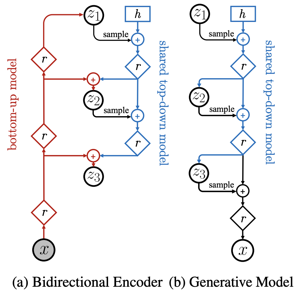
Figure 2: The neural networks implementing an encoder and generative model. (Vahdat & Kautz, 2020)
NVAE는 latent groups $z = \{z_1, z_2, … z_L\}$에 대해 $q(z|x) = \Pi_l q(z_l|z_{<1}, x)$의 hierarchical approximate posterior를 활용한다. ELBO는 다음과 같다.
$$\mathcal L_{VAE}(x) = \mathbb E_{q(z|x)}[\log p(x|z)] - D_{KL}(q(z_1|x)||p(z_1)) - \sum^L_{l=2}\mathbb E_{q(z_{<l}|x)}[D_{KL}(q(z_l|x, z_{<l})||p(z_l))]$$
Encoder가 이미지로부터 feature map r를 생성(i.e. hierarchical approximate posterior, $q(z_l|x, z_{<l})$), Decoder가 trainable basis h로부터 Encoder feature map을 역순으로 더해가며 이미지를 생성하는 U-Net 구조를 상상하자. Generation 단계에서는 Encoder feature map r이 주어지지 않기에, feature map의 prior distribution $p(z_l)$의 샘플로 대체한다. 이는 어찌 보면 Spatial noise를 더해가는 StyleGAN[Karras et al., 2018.]과도 형태가 유사하다.
다만 이 경우, $D_{KL}$의 조기 수렴에 따라 posterior collapse가 발생할 가능성이 높기에, 여러 engineering trick이 함께 제안되었다. Decoder에는 Depthwise-seperable convolution을 활용하지만 Encoder에서는 사용하지 않고, SE Block[Hu et al., 2017.]과 Spectral regularization, KL Warmup 도입, Batch normalization의 momentum parameter 조정 등이 있다.
이를 통해 당시 Normalizing Flows와 VAE 계열 모델 중에서는 좋은 성능을 보였다. 하지만 논문에서는 NLL(bit/dim)에 관한 지표만 보일 뿐, FID나 Precision/Recall 등 지표는 보이지 않아 다른 모델과의 비교는 쉽지 않았다.
정성적으로 보았을 때는 NVAE는 여전히 다소 Blurry 한 이미지를 보이거나, 인체의 형태가 종종 왜곡되는 등의 Degenerate Mode가 관찰되며 아쉬운 모습을 보이기도 했다.
Normalizing Flows
- RealNVP: Density estimation using Real NVP, Dinh et al., 2016. [arXiv:1605.08803]
VAE가 연구되는 동시에 approximate posterior 도입 없이 marginal $\log p_{\theta,X}(x)$를 구하려는 시도가 있었다.
만약 parametrized generator $G_\theta: Z \to X$가 가역함수 (혹은 전단사함수, Bijective)이면 marginal pdf는 변수 치환 법칙에 따라 $p_{\theta,X}(x) = p_Z(f^{-1}(x))\left|\frac{\partial f^{-1}(x)}{\partial x}\right|$를 만족한다.
적분 없이도 determinant of jacobian을 구함으로 marginal을 구할 수 있게 되었고, 이 과정이 differentiable 하다면 gradient 기반의 학습도 가능하다. 문제는 뉴럴 네트워크 가정에서 jacobian을 구한 후, 이미지 pixel-dimension에서 $O(n^3)$의 determinant 연산을 수행해야 한다는 것이다 (e.g. 256x256 이미지의 경우 281조, 281 Trillion).
RealNVP는 현실적인 시간 내에 이를 수행하기 위해 Coupling layer를 제안한다.
$$\begin{align*} y_{1:d} &= x_{1:d} \\ y_{d+1:D} &= x_{d+1:D} \odot \exp(s_\theta(x_{1:d})) + t_\theta(x_{1:d}) \end{align*}$$
Affine coupling layer는 hidden state를 반으로 나눠 한 쪽을 유지한 채, 나머지 반에 다른 반을 기반으로 affine transform을 가한다. 이는 가역 연산으로, 절반의 원본을 통해 다른 절반의 역연산이 가능하며, 연산 복잡도 역시 순연산과 동일하다.
$$\begin{align*} x’_{1:d} &= y _{1:d} \\ x’ _{d+1:D} &= (y _{d+1:D} - t _\theta(y _{1:d})) \odot \exp(-s _\theta(y _{1:d})) \end{align*}$$
Affine coupling layer의 Jacobian matrix는 $y_{1:d}$와 $x_{1:d}$가 identity mapping이기에 identity block matrix를 형성, $y_{1:d}$는 $x_{d+1:D}$에 dependent 하지 않기 때문에 zeroing out 되고, $y_{d+1:D}$와 $x_{d+1:D}$는 element-wise linear 관계로 diagonal block matrix가 되어, 최종 low triangular matrix의 형태로 구성된다. 이 경우 determinant는 별도의 matrix transform을 거치지 않고 대각 원소의 곱으로 곧장 연산해 낼 수 있다.
$$\begin{align*} \frac{\partial y}{\partial x} &= \left[\begin{matrix} \mathbb I_d & 0 \\ \frac{\partial y_{d+1:D}}{\partial x_{1:d}} & \mathrm{diag}[\exp(s(x_{1:d}))] \end{matrix}\right] \\ \det\frac{\partial y}{\partial x} &= \prod_{i=d+1}^D \exp(s_i(x_{1:d})) = \exp\left(\sum^D_{i=d+1}s_i(x_{1:d})\right) \end{align*} $$
Affine coupling layer를 여러 개 쌓아 $f_2(f_1(z))$의 형태로 표현한다면, 역함수는 $f_1^{-1}(f_2^{-1}(x))$로 네트워크를 출력부부터 역순으로 연산해 나가면 되고, determinant 역시 각각 계산하여 구할 수 있다.
$$\det\frac{\partial f_2}{\partial z} = \det\left(\frac{\partial f_2}{\partial f_1}\frac{\partial f_1}{\partial z}\right) = \left(\det \frac{\partial f_2}{\partial f_1}\right)\left(\det\frac{\partial f_1}{\partial z}\right)$$
다만 이 경우 한쪽에만 연산이 가해지는 형태이기에, Coupling layer 이후 shuffling $[y_{1:d}, y_{d+1:D}] = [x_{d+1:D}, x_{1:d}]$를 수행하여 각각의 청크가 모두 transform 될 수 있도록 구성한다.
$$\begin{align*} \max_\theta \log p_{\theta, X}(x) &= \max_\theta \left[\log p_Z(f_\theta^{-1}(x)) + \log\left|\det\frac{\partial f_\theta^{-1}(x)}{\partial x}\right|\right] \\ &= \max_\theta \left[\log p_Z(f_\theta^{-1}(z)) - \exp\left(\sum^L_{l=1}\sum^D_{i=d+1}s^l_{\theta,i}(x^l_{1:d})\right)\right] \end{align*}$$
L개 affine coupling layer w/shuffling으로 구성된 네트워크 $f_\theta$의 최종 objective는 위와 같다.
Normalizing Flow는 Network의 형태를 제약함으로 Generation과 함께 exact likelihood를 구할 수 있게 되었고, 별도의 Encoder 없이 posterior를 구할 수 있다는 장점이 있다.
하지만 반대로, 네트워크의 형태에 제약을 가하기에 발생하는 approximation의 한계가 발생할 수 있다. 자세한 내용은 뒤에서 논의한다.
- Glow: Generative Flow and Invertible 1x1 Convolutions, Kingma & Dhariwal, 2018. [arXiv:1807.03039]
Glow는 이에서 더 나아가, 256x256 크기의 이미지까지 연구를 확장하여 그 실용성을 보였다.
기본적으로 가역 함수와 치환 법칙을 기저로 하며, RealNVP에서 몇 가지 네트워크 구조를 수정하였다.
가장 먼저 Batch Normalization을 Activation Normalization으로 교체한다. 당시 GPU VRAM은 10GB (1080Ti, 2080Ti) 정도로, 이미지의 크기가 조금만 커져도 배치의 크기를 1~2까지로 줄여나가야 했다. 이러한 상황에서 BN의 Moving statistics는 noisy 했고, 성능 하락을 감안해야 했다.
이에 Glow는 최초 Forward pass에서 normalization 직전 레이어의 평균과 표준편차를 연산하여 저장해 두고, 이를 토대로 normalization을 수행한다. 한 번 초기화된 파라미터는 이후 별도의 이동 평균 처리나 통계치 재연산을 수행하지 않고, 일반적인 trainable constant로 여긴다. 이를 Data-Dependent Initalization (DDI)이라 하고, 위 정규화 레이어를 activation normalization이라 한다.
# PSEUDO CODE OF DATA-DEPENDENT INITIALIZATION
def __init__(self):
    super().__init__()
    self.mean, self.logstd = None, None

def forward(self, x: Tensor) -> tuple[Tensor, Tensor]:
    # x: [B, C, H, W]
    if self.mean is None:
        with no_grad():
            self.register_parameter(
                "mean",
                nn.Parameter(x.mean(dim=[0, 2, 3], keepdim=True)),
            )
            self.register_parameter(
                "logstd",
                nn.Parameter(x.std(dim=[0, 2, 3], keepdim=True).log()),
            )
    norm = (x - self.mean) * (-self.logstd).exp()
    logdet = -self.logstd
    return norm, logdet

def inverse(self, y: Tensor) -> Tensor:
    assert self.mean is not None
    return y * self.logstd.exp() + self.mean
ActNorm은 첫 배치에서 zero-mean, unit-variance의 feature map을 반환하여 학습을 안정화하고, 이후는 학습에 따라 자연스레 값을 바꿔나간다.
FYI. DDI는 Weight normalization[Salimans & Kingma, 2016.]에서 효과가 확인된 바 있다.
다음은 Invertible 1x1 convolution이다. RealNVP가 Shuffling을 통해 절반의 feature map에 연산이 가해지지 않던 문제를 해결했다면, Glow는 가역 행렬을 channel-axis에 곱함으로(1x1 conv), 채널 축의 정보 공유를 학습 가능하도록 두었다(generalized permutation).
우선 초기화 단계에서 QR 분해를 통해 1x1 Convolution의 Random weight matrix W가 invertible 하게 두었고, 이후에는 $\log|\det W|$를 직접 연산하여 objective에 활용(torch.linalg.slogdet), inference에는 weight의 역행렬을 구하여 활용한다(torch.linalg.inv).
다만 이 경우 channel-axis의 크기가 커질 경우 연산량에 부담이 생길 수 있으므로, 다음과 같이 LU Decomposition을 활용하여 연산량을 줄여볼 수도 있다.
def __init__(self, channels: int):
    super().__init__()
    weight, _ = torch.linalg.qr(torch.randn(channels, channels))
    p, l, u = torch.linalg.lu(weight)
    self.p = nn.Parameter(p)
    self.l = nn.Parameter(l)
    self.u = nn.Parameter(u)
    self.s = nn.Parameter(torch.diagonal(u))
    self.register_buffer("i", torch.eye(channels), persistent=False)

@property
def weight(self):
    return self.p @ (self.l.tril(-1) + self.i) @ (self.u.triu(1) + self.s)

def forward(self, x: torch.Tensor) -> tuple[torch.Tensor, torch.Tensor]:
    b, c, h, w = x.shape
    shuffled = F.conv2d(x, self.weight[..., None, None])
    logdet = self.s.abs().log().sum() * h * w
    return shuffled, logdet

def inverse(self, y: torch.Tensor) -> torch.Tensor:
    return F.conv2d(x, torch.linalg.inv(self.weight)[..., None, None])
마지막으로 affine coupling layer 두 개 네트워크 $t_\theta, s_\theta$의 마지막 convolution 레이어를 zero-initialize 하여 학습의 첫 forward pass에서는 identity mapping이 되도록 구성하였다. 이는 LayerScale[Touvron et al., 2021.]처럼 레이어가 많은 네트워크를 운용할 때 학습을 안정화한다고 알려져 있다.
이러한 트릭을 활용하여 Glow는 256x256 이미지에서도 좋은 합성 결과를 보였고, 아직도 likelihood 기반의 새로운 학습 방법론이 소개될 때마다 베이스라인으로 인용되고 있다.
- CIF: Relaxing Bijectivity Constraints with Continuously Indexed Normalising Flows, Cornish et al., 2019. [arXiv:1909.13833]
앞서 이야기한 Bijective의 제약에 의해 발생하는 Approximation의 한계에 관하여 이야기해 보고자 한다.
Exact Support Matching
Normalizing flows는 대표적인 pushforward measure이다.
i.e. measurable space $(Z, \Sigma_Z, \mu_Z)$, $(X, \Sigma_X)$와 measurable mapping $f: Z \to X$에 대해 $f_\# p_Z = p_Z(f^{-1}(B)); B \in \Sigma_X$를 Pushforward measure라 한다. (w/sigma algebra $\Sigma_Z, \Sigma_X$ of $Z, X$)
Normalizing flows는 특히 generator $f$를 전단사함수로 가정하기 때문에, $\mathrm{supp}\ p_X$와 $\overline{f(\mathrm{supp}\ p_Z)}$가 같아야 한다. i.e. support of $p_X$: $\mathrm{supp}\ p_X = \{x \in X : \forall \mathrm{open}\ U \ni x,\ p_X(U) > 0 \}$, closure of $S$: $\overline S$
FYI. 직관적으로 support는 사건의 발생 확률이 0보다 큰 원소의 집합이다. 확률이 존재하는 공간을 전단사 함수로 대응하였을 때, 대응된 원소 역시 발생 가능성이 0보다 커야 함을 의미한다.
RealNVP, Glow 등의 Normlizing flows는 대부분 연속 함수이다(tanh, relu, sigmoid 등의 연속 활성함수를 사용하는 네트워크 기반의 affine coupling을 가정). 동시에 전단사 함수이기 때문에 역함수 역시 연속 함수이고, 이 경우 $f$는 topological property를 보존하는 homeomorphism이다(위상 동형 사상).
위상 동형인 $Z$와 $X$는 hole의 수, connected component의 수 등이 같아야 한다. 흔히 가정하는 정규 분포의 support는 hole을 가지지 않고, 1개의 connected components를 가진다. 만약 데이터의 분포가 두 Truncate Normal 분포의 mixture로 표현되어 그의 support가 2개의 connected components를 가진다면, 두 분포를 대응하는 연속 함수 형태의 normalizing flows를 construction 하는 데에 한계가 발생한다.
Lipschitz Constraints
경우에 따라 Invertible ResNet[Behrmann et al., 2018.], Residual Flow[Chen et al., 2019.]는 invertibility를 위해 network의 lipschitz constant를 제약한다.
$$\mathrm{Lip}(f) = \sup_{x\ne y}\frac{|f(x) - f(y)|}{|x - y|} \implies |f(x) - f(y)| \le \mathrm{Lip}(f)|x - y|\ \forall x, y$$
Injective $f$에 대해 bi-Lipschitz constant $\mathrm{BiLip}\ f = \max\left(\sup_{z\in Z}|J_{f(z)}|, \sup_{x\in f(Z)}|J_{f^{-1}(x)}|\right)$를 정의하자 (w/norm of jacobian $|J_\cdot|$). Homeomorphic 하지 않은 두 topological space $Z$와 $X$는 $\lim_{n\to\infty}\mathrm{BiLip}\ f_n = \infty$일 때에만 $(f_{n})_\#p_Z \stackrel{D}{\to}p_X$의 weak convergence를 보장한다(under statistical divergence $D$, i.e. $D((f_n) _\#p_Z, p_X)\to 0$ as $n\to\infty$).
Residual Flow의 각 레이어가 Lipschitz Constant $K$를 갖는다면, N개 레이어로 구성된 네트워크 전체의 Lipschitz Constant는 최대 $K^N$이다. Homeomorphic 하지 않은 임의의 pushforward measure $(f_n)_\#p_Z$를 $p_X$로 근사하기 위해서는 $K^N\to\infty$의 조건이 만족해야 하고, 그에 따라 무수히 많은 레이어를 요구할 수도 있다.
Normalizing flows는 네트워크의 제약상 고질적으로 Exact support matching 문제와 Lipschitz-constrained network의 표현력 문제를 겪게 된다. Continuously Indexed Flow, CIF는 이를 해결하고자 augmentation을 제안한다.
CIF는 bijective generator $G_\theta$를 indexed family $\{F_{\theta, u}(\cdot): Z \to X\}_{u\in\mathrm{supp}\ U}$ 로 확장한다. $x = F _\theta(z, u)$의 2 변수 함수를 생각한다면, u가 고정되어 있을 때, $z = F _\theta^{-1}(x; u)$의 가역함수를 고려할 수 있다. $z$와 $x$는 여전히 change-of-variables의 관계인 반면, $u\sim U$는 데이터의 차원과 무관한 잠재 변수이기에 variational inference의 대상이 된다.
prior $p_U(u)$와 approximate posterior $q_\phi(u|x)$를 가정하자. 우리의 목표는 $p_{\theta, X}(x)$이고, graphical model을 가정할 때 joint는 $p_{\theta, X,U}(x, u) = p_U(u)p_Z(F^{-1}_\theta(x; u))\left|\frac{\partial F^{-1} _\theta(x)}{\partial x}\right|$이다. variational lowerbound는 다음과 같이 정리된다.
$$\mathrm E _{u\sim q _\phi(u|x)}\log\frac{p _{\theta, X,U}(x, u)}{q _\phi(u|x)} = \mathbb E _{u\sim q _\phi(u|x)}\left[\log p _U(u) + \log\frac{p_Z(F^{-1} _\theta(x; u))}{q _\phi(u|x)}\right] + \log\left|\det\frac{\partial F^{-1} _\theta(x)}{\partial x}\right|$$
CIF는 여기서 더 발전시켜, prior $p_U(u)$를 $z$ 조건부 분포 $p_{\theta, U|Z}(u|z) = \mathcal N(\mu_\theta(z), \Sigma_\theta(z))$로 두어 학습의 대상으로 삼는다(i.e. $p_{\theta, X, U}(F_\theta(z; u), u) = p_{\theta, U|Z}(u|z)p_Z(z)|J_{F^{-1}_\theta}|$).
이를 통해 저자는 homeomorphic 하지 않은 두 공간에 대해서도 $F_\theta$가 $Z$에서 $U$에 대해 항상 Surjective이면, CIF가 Exact support matching을 가능케 함을 보인다. lipschitz constraints가 존재하는 네트워크에서도 동일하다.
$$\forall z\in\mathrm{supp}\ Z,\ F_\theta(z; \cdot): U\to X\ \mathrm{is\ surjective} \iff p_{\theta, X} = p_X$$
Surjective라는 어렵지 않은 조건 내에서 exact match가 가능한 해가 존재함을 보였고, 이의 학습 가능성은 emperical 하게 NLL이 낮아짐을 통해 보인다.
이렇게 Normalizing flows에서 데이터의 차원을 넘어 새로운 latent variable을 추가하는 형태를 agumentation이라 하고, ANF[Huang et al., 2020.], VFLow[Chen et al., 2020.]의 Concurrent work가 존재한다.
이 두 논문 모두 augmented normalizing flow에 관한 emperical study를 보이며, VFlow의 경우 CIF와 유사히 augmented normalizing flow가 vanilla보다 NLL이 더 낮을 수 있음을 보인다.
Continuous Normalizing Flows
앞서 확인하였듯, Normalizing Flows는 네트워크의 Lipschitz Constant가 제약되었을 때 임의 분포의 근사를 위해 레이어의 수를 무한히 요구할 수 있다. 그렇다면 레이어의 수를 무한히 표현하기 위해서는 어떻게 해야 할까.
두 집합 $Z, X\subset\mathbb R^D$을 연관 짓는 함수 $F_\theta: Z\to X$가 있다 가정하자. 함수 $F_\theta$는 N-Layer Residual Network로, $z\in Z$를 입력으로 값을 순차적으로 변환시켜 끝에 $X$에 도달하게 한다. 이에 $F_\theta$의 i번째 레이어 $f^{(i)}_ \theta = f_ \theta(\cdot; i)$를 $f_\theta(\cdot; t_i)$로 표현하면, $x_{t_{i+1}} = x_{t_i} + f_\theta(x_{t_i}; t_i)$이고, $f_\theta: \mathbb R^D\times I\to\mathbb R^D$이다.
($t_i = i / N,\ i = 0,1,…,N\implies I = \{t_i\}_{i=0}^{N-1};\ x_0 = z,\ x_1\in X$)
$Nf_\theta(x_{t_i}; t_i) = N(x_{t_{i+1}} - x_{t_i})$에 대해 $N\to\infty$를 상정하면, 극한이 존재할 때 다음과 같이 모델링할 수 있다.
$$\lim_{\Delta t := N^{-1}\to 0}\frac{x_{t + \Delta t} - x_{t}}{\Delta t} = \frac{dx_t}{dt} = f_\theta(x_t; t): \mathbb R^D\times[0, 1]\to\mathbb R^D \\ x_1 - x_0 = \int^1_0\frac{dx_t}{dt}dt = \int^1_0 f_\theta(x_t; t)dt\implies x_1 = x_0 + \int^1_0f_\theta(x_t; t)dt$$
$N\to\infty$ 이므로 레이어 $f^{(i)}_ \theta$의 첨자에 해당하던 $I$는 $[0, 1)$의 구간으로 표현되고, 이제는 N번째 hidden layer가 아닌 어떤 순간 $t$의 $x_t$ 변량 $dx_t/dt$를 $f_ \theta(x_t; t)$의 time-conditional neural network로 표현한다.
각 레이어가 서로 독립된 Subnetwork로 구성되던 기존과 달리, 이제는 모든 시점에서 하나의 네트워크를 공유하고, 대신 현시점 $t\in[0, 1]$를 조건으로 주는 방식이다.
$f_\theta$가 특수한 형태로 제약되지 않는 이상 적분을 포함한 mapping은 불가능하므로, Euler solver, Runge-Kutta Method 등 Numerical solver를 통해 근사한다. 이 경우 사전에 Discretized points $\{t_i\}_{i=1}^N$를 정의해 두었다가, 다음과 같이 1st-order approximate 하는 예시를 들 수 있다.
$$x_{t_{i+1}} = x_{t_i} + (t_{i+1} - t_i)f_\theta(x_{t_i}; t_i);\ \ x_{t_0} = z,\ x_{t_N} = x$$
문제는 어떻게 $f_\theta(x_t; t)$를 학습할 것인지이다.
- NODE: Neural Ordinary Differential Equations, Chen et al., 2018. [arXiv:1806.07366]
Neural ODE(이하 NODE)는 이에 대한 Practical solution을 제안한다.
평소와 같이 Mapping result $x_1$에 대해 loss objective $L(x_1)$을 취해 gradient 기반 optimization을 수행한다고 가정하자. 이때 적분은 Numerical ODE Solver로 대체한다.
$$L(x_1) = L\left(x_0 + \int_0^1 f_\theta(x_t; t)dt\right) \approx L(\text{ODESolve}(f_\theta, x_0))$$
우리가 필요한 것은 초기값 업데이트를 위한 $\partial L/\partial x_0$와 네트워크 업데이트를 위한 $\partial L/\partial\theta$이다.
가장 먼저 Loss objective $L$에 각 variable $x_t$의 기여량 $a_t = \partial L/\partial x_t$를 정의한다. 이를 Adjoint라 하자. $x_{t+1} = x_t + \Delta t f_\theta(x_t; t)$일 때 Adjoint의 변량은 또 다른 ODE로 표현된다.
$$\begin{align*} a_t &= \frac{\partial L}{\partial x_t} = \frac{\partial L}{\partial x_{t+1}}\frac{\partial x_{t+1}}{\partial x_t} = a_{t+1}\frac{\partial x_{t+1}}{\partial x_t} = a_{t+1}\left(1 + \Delta t\frac{\partial f_\theta(x_t; t)}{\partial x_t}\right) \\ \frac{da_t}{dt} &= \lim_{\Delta t \to 0}\frac{a_{t+1} - a_t}{\Delta t} = \lim_{\Delta t \to 0}-a_{t+1}\frac{\partial f_\theta(x_t; t)}{\partial x_t} = -a_t\frac{\partial f_\theta(x_t; t)}{\partial x_t} \end{align*}$$
이를 1부터 0까지 적분하면 $\partial L / \partial x_0$와 동치이고, 동일 논리로 $\partial L/\partial \theta$도 구할 수 있다.
$$\frac{\partial L}{\partial\theta} = \sum a_{k+1}\frac{\partial x_{k+1}}{\partial\theta} = \sum a_{k+1}\frac{\partial f_\theta(x_k; t_k)}{\partial \theta}\Delta t \to \int^1_0 a_t\frac{\partial f_\theta(x_t; t)}{\partial \theta} dt \\ \implies \frac{dL}{dx_0} = -\int^0_1 a_t\frac{\partial f_\theta(x_t; t)}{\partial x_t}dt + a_1,\ \frac{dL}{d\theta} = -\int^0_1a_t\frac{\partial f_\theta(x_t; t)}{\partial\theta}dt\\ \implies \left[\begin{matrix}\frac{\partial L}{\partial x_0} \\ \frac{\partial L}{\partial\theta}\end{matrix}\right] = \left[\begin{matrix}\frac{\partial L}{\partial x_1} \\ 0\end{matrix}\right] + \int^0_1\left[\begin{matrix} -a_t\frac{\partial f_\theta(x_t; t)}{\partial x_t} \\ -a_t\frac{\partial f_\theta(x_t; t)}{\partial \theta} \end{matrix}\right]dt$$
구해낸 Gradient 또한 적분을 포함한 형태이므로 Numerical solver를 통해 근사한다. Numerical solver는 각 시점마다 JVP 연산을 통해 $f_\theta$의 derivative와 $a_t$를 곱하여 step gradient를 연산하고, 이를 누적하는 방식으로 실제 gradient를 근사해 나간다. 이를 Adjoint sensitivity method라 한다.
만약 Loss objective $L$로 Mean Maximum Discrepancy를 상정한다면, 우리는 Adjoint sensitivity method를 통해 분포를 학습할 수 있다[Dziugaite et al., 2015.].
Normalizing flows는 반대로 Change-of-variables를 통해 exact likelihood를 maximizing 하는 방식으로 학습을 수행한다. NODE는 Adjoint method와 동일한 논리로 Instantaneous change of variables $\partial \log p(x_t)/\partial t$를 제안하고, 이를 적분하는 방식으로 likelihood를 획득한다.
$$\log p(x_1) = \log p(x_0) + \int^1_0\frac{\partial \log p(x_t)}{\partial t}dt; \frac{\partial\log p(x_t)}{\partial t} = -\text{Tr}\left(\frac{df_\theta(x_t; t)}{dx_t}\right)$$
FYI. $f_\theta(x_t; t)$가 Lipschitz continuous일 때 $f_\theta$가 모든 $t$에 대해 유일한 값을 가지고-invertible 해지므로, 가역함수를 기반으로 한 change-of-variables의 유효성을 위해 $f_\theta$에는 주로 Lipschitz continous 조건이 부여된다.
이렇게 log-likliehood를 얻었다면, expectation을 취해 Loss objective로 정의하고, adjoint method를 통해 gradient를 획득해 네트워크를 업데이트한다. Jacobian의 trace를 현실적인 시간 내에 얻기 위해서는 마찬가지로 network architecture를 특수한 형태로 정하는 등의 제약이 가해진다.
$x_{t + \Delta t} = T(x_t) = x_t + f_\theta(x_t; t)\Delta t$를 가정. $p_{t + \Delta t} = p_t(T^{-1}(x_t))|\det (J_{T^{-1}}(z))|$의 Change-of-variables에 대해 $T^{-1}(z) = z - f_\theta(z; t)\Delta t$이고, Jacobian은 다음으로 정리: $J_{T^{-1}}(z) = I - \frac{\partial f_\theta(z; t)}{\partial z}\Delta t$. Jacobi’s fomula에 의해 $\det(I + \Delta t A) = 1 + \text{Tr}(A)\Delta t + o(\Delta t)$이므로, $|\det(J_{T^{-1}}(z))| = 1 - \text{Tr}\left(\frac{\partial f_\theta(z; t)}{\partial z}\right)\Delta t + o(\Delta t)$ 표현상 편의를 위해 $\text{Tr}\left(\frac{\partial f_\theta(z; t)}{\partial z}\right)$를 divergence $\operatorname{div}f$로 표기. $$\begin{align*}
p_{t + \Delta t}(z) &= p_t(z - f_\theta(z; t)\Delta t)\left[1 - \operatorname{div}f\cdot\Delta t\right] + o(\Delta t) \\
&= [p _t(z) - f _\theta(z; t)^T\nabla p_t(z)\Delta t]\left[1 - \operatorname{div}f\cdot\Delta t\right] + o(\Delta t) \\
&= p _ t(z) - [f _ \theta(z; t)^T\nabla p _ t(z) + p _ t(z)\operatorname{div}f]\Delta t + o(\Delta t) \\
&= p _t(z) - \nabla\cdot [p _t(z)f _\theta(z; t)]\Delta t + o(\Delta t)\\
\implies & \frac{\partial p _t(z)}{\partial t} = -\nabla\cdot [p _t(z)f _\theta(z; t)]\\
\implies & \frac{\partial}{\partial t}\log p _t(z) = -\frac{1}{p _t(z)}\nabla\cdot [p _t(z)f _\theta(z; t)] = -\operatorname{div}f \end{align*}$$ FYI. Taylor appximation w/Jacobi’s formula
$$\begin{align*}
&\frac{d}{d\epsilon}\det M_\epsilon = \det M_\epsilon\cdot\operatorname{Tr}(M_\epsilon^{-1}M’_\epsilon) & \text{Jacobi’s formula} \\
&\implies \frac{d}{d\epsilon}\det(1 + \epsilon A)| _{\epsilon = 0} = \det I\cdot \operatorname{Tr}(I^{-1}A) = \operatorname{Tr}(A)\\
&\implies \det (I + \epsilon A)\approx \det(I) + \epsilon\operatorname{Tr}(A) & \because \text{Taylor approximation}
\end{align*}$$pf. Instantaneous change of variables
- FFJORD: Free-form Continuous Dynamics for Scalable Reversible Generative Models, Grathwohl et al., 2018. [arXiv:1810.01367]
FFJORD는 네트워크에 가해지는 제약 없이 Trace of Jacobian의 계산 비용을 추가로 줄이기 위해 Hutchinson Trace Estimation Method $\mathrm{Tr}(A) = \mathbb E_{\epsilon\sim\mathcal N(0, I)}[\epsilon^TA\epsilon]$를 활용한다.
$$\begin{align*} \log p(x_1) &= \log p(x_0) - \int^1_0\mathrm{Tr}\left(\frac{df_\theta(x_t; t)}{dx_t}\right) \\ &= \log p(x_0) - \mathbb E_{\epsilon\sim \mathcal N(0, I)}\left[\int^1_0\epsilon^T\frac{df_\theta(x_t; t)}{dx_t}\epsilon\right] \end{align*}$$
VAE 당시와 마찬가지로 $\epsilon\sim \mathcal N(0, I)$에 대한 Expectation 연산은 각 1개 표본만을 활용하였고, 대신 배치 크기를 Tabular 데이터셋에서는 10,000개, 이미지 데이터셋에서는 900개로 구성하였다.
또한, Hutchinson estimation $\mathrm{Tr}(A)$의 분산이 $||A||_F$에 따라 증가한다는 점에 착안하여, 네트워크에 Bottleneck layer가 있는 경우 (i.e., $f = g\circ h$ for $h(x)\in \mathbb R^H$, $x\in \mathbb R^D$, and $H< D$), 연산을 재정렬하는 방식으로 Dimension을 줄여 $||A|| _F$와 함께 Estimation variance를 줄이는 방식을 채택한다.
$$\mathrm{Tr}\left(\frac{df}{dx}\right) = \mathrm{Tr}\bigg(\underbrace{\frac{dg}{dh}\frac{dh}{dx}}_{\mathbb R^{D\times D}}\bigg) = \mathrm{Tr}\bigg(\underbrace{\frac{dh}{dx}\frac{dg}{dh}} _{\mathbb R^{H\times H}}\bigg)$$
실제로 이러한 분산 감소는 학습 속도의 개선으로도 이어졌다고 보여진다. $J=df_\theta/dx_t$에 대해 Trace term은 $\epsilon^TJ$를 Vector-Jacobian Product (VJP) 연산을 통해 획득한 후, $\epsilon$을 추가로 곱하는 방식으로 근사하게 된다. 최종 Adjoint method를 통해 maximizing likelihood의 방식으로 생성 모델을 학습한다.
비록 네트워크의 형태에 가해지는 제약을 해소하면서도 효율적인 Trace estimation을 보였지만, 학습 중 ODE Solver를 수반해야 하는 Adjoint method의 한계상 학습과 추론 속도의 한계점은 해소되지 못했다.
EBM: Energy-based Model
우리는 지금까지 Likelihood $p_X(x)$를 미분 가능한 형태로 계산하거나 근사하고, 이를 토대로 학습을 수행해 왔다. Approximate posterior를 활용해 log-likelihood의 하한을 정의하기도 하고, Bijective generator를 통해 $X$-space likelihood를 $Z$-space에서 연산하기도 했다.
실상 $p_X$의 연산을 어렵게 하는 것은 꾸준히 적분의 문제였다. 특히 앞선 상황에서는 대개 $z\mapsto x$의 generator를 두고, $p_\theta(x) = \int_Z p(z)p_\theta(x|z)dx$로 정의된 likelihood를 추정하는 과정에서 발생하는 $Z$-space 적분 문제에 대해 다뤄왔다.
반대로 $z$ 없이 $p_X(x)$를 직접 추정하는 방식도 재고하자. 만약 우리가 $p_{\theta,X}(x)$를 추정할 수 있다면, 네트워크가 직접 샘플을 생성하진 않더라도 샘플링 방법론 (e.g., MCMC)을 통해 known proposal distribution (or prior) $p_Z(z)$에서부터 $p_X(x)$에 적합한 샘플을 찾아나갈 수 있을 것이다.
네트워크가 어떤 positive scalar $\tilde p_\theta(x)$를 출력한다 가정하자. 확률 함수의 조건상 $X$-space 적분이 1이어야 하므로, $\tilde p_\theta$는 normalizing 된 후에 density function으로 이용될 수 있다.
$$p_\theta(x) = \frac{\tilde p_\theta(x)}{Z_\theta},\quad Z_\theta = \int_X \tilde p_\theta(x)dx$$
여전히 문제는 적분이다. 현재의 일차적 목표는 분모의 적분항 $Z_\theta$ (i.e., partition function)을 우회하며 unnormalized density $\tilde p_\theta$를 학습하는 것이다. EBM은 이에 대해 Contrastive Divergence라는 해결책을 내놓는다.
- Training Products of Experts by Minimizing Contrastive Divergence, Hinton, 2002.
- Energy-Based Models for Sparse Overcomplete Representations, Teh et al., JMLR 2003.
Energy-based Model (EBM)은 분포를 Gibbs distribution (i.e., Boltzmann distribution)으로 바라본다. Energy function $E_\theta(x)$에 대해 unnormalized density가 $\tilde p_\theta(x) = \exp(-E_\theta(x))$를 따른다고 하자. 우리의 목표는 어떤 상태 혹은 데이터 $x$가 주어졌을 때, 이의 발생 가능성 (likelihood)를 partition function에 우회적으로 추정하는 것이다. 이 분포의 maximizing log-likelihood를 가정하자.
$$\log p_\theta(x) = \log \frac{\exp(-E_\theta(x))}{Z_\theta} = -E_\theta(x) - \log Z_\theta$$
Likelihood 학습을 위한 $\theta$-gradient는 다음과 같다.
$$\begin{align*} \nabla_\theta\log p_\theta(x) &= -\nabla_\theta E_\theta(x) - \nabla_\theta\log Z_\theta = -\nabla_\theta E_\theta(x) - \frac{\nabla_\theta Z_\theta}{Z_\theta} \\ &= -\nabla_\theta E_\theta(x)- \frac{1}{Z_\theta}\int_X \nabla_\theta \exp(-E_\theta(x’))dx’ \\ &= - \nabla_\theta E_\theta(x) + \int_X\frac{\exp(-E_\theta(x’))}{Z_\theta}\nabla_\theta E_\theta(x’)dx’ \\ &= -\nabla_\theta E_\theta(x) + \mathbb E_{x’\sim p_\theta(x)}[\nabla_\theta E_\theta(x’)] \end{align*}$$
결과적으로 $\nabla_\theta\mathbb E_{x\sim p_X}[\log p_\theta(x)]= - \mathbb E_{x\sim p_X}[\nabla_\theta E_\theta(x)] + \mathbb E_{x’\sim p_\theta}[\nabla_\theta E_\theta(x’)]$이고, Energy function을 각각 데이터 분포 $p_X$와 $E_\theta$에 의해 형성된 분포 $p_\theta$에서 평가함을 의미한다.
$$\mathcal L = -\mathbb E_{x\sim p_X}[E_\theta(x)] + \mathbb E_{x’\sim p_{\theta^-}}[E_\theta(x’)],\quad \theta^- = \mathrm{stop\text{-}grad}(\theta)$$
이러한 형태의 목적함수를 Contrastive divergence라고 하고, partition function 없이도 log-likelihood를 maximizing 하는 Energy function $E_\theta$의 학습이 가능해졌다. 적분 없이도 데이터의 가능도를 학습할 수 있게 된 것이다.
학습을 위해서는 $E_\theta$로 정의되는 $p_\theta(x’) = \exp(-E_\theta(x’)) / Z_\theta$로부터 표본을 획득할 수 있어야 한다. Rejection Sampling, MH (Metropolis Hastings) 등의 MCMC (Monte Carlo Markov Chain) 방법론은 partition function을 모르는 경우에도 샘플링을 수행할 수 있다. 특히 MH의 경우는 proposed sample과 previous sample의 density ratio를 추정하기 때문에 자연스레 partition function이 canceling 되어 $E_\theta$만으로도 표본 추출이 가능하다.
다만, 이 경우 MCMC 샘플링 자체의 비용과 분산 문제를 우회하기 위해, Teh et al., JMLR 2003. 에서는 Markov chain을 실제 데이터 샘플에서 시작하도록 하였다. 이는 MCMC가 undesired mode에 빠지는 것을 방지하고, EBM이 근사하고자 하는 데이터 표본에서 시작함으로, 근사에 필요한 표본의 수와 분산을 줄이고자 하였다.
그럼에도 학습 중간의 multiple-forward를 요구하는 샘플링 과정은 연산상 부담으로 남아 있었다. 이는 이후 single-forward generation을 가정하는 모델들이 샘플링 부담을 줄이면서도 generated sample에 대한 평가를 가능케 한다는 점에서, Contrastive learning이라는 토픽으로 확장되어 현재도 활발히 활용되고 있다.
Score Matching
Partition function을 배제하고 분포를 추정하기 위해 경우에 따라서는 Score function을 정의하기도 한다. Log-likelihood $\log p_\theta(x) = \log\tilde p_\theta(x) - \log Z_\theta$에 대한 $x$-미분을 상정하자. 이때 $Z_\theta$는 $x$에 무관한 상수이므로 미분 과정에서 소실된다.
$$s_\theta(x) := \nabla _x \log p _\theta(x) = \nabla _x\log \tilde p _\theta(x) - \cancel{\nabla _x\log Z _\theta}$$
이렇게 미분 연산자를 통해 적분항을 제거한 형태를 Score function $s _\theta(x) = \nabla _x\log p _\theta(x)$이라고 한다. EBM의 가정에서는 $s _\theta(x) = -\nabla_x E _\theta(x)$와 동치이다. 초기 Score matching은 여전히 network output이 unnormalized density이고, 이의 gradient를 직접 추정하는 방식으로 score를 계산해 왔다. 이는 score가 아닌 density를 유지함으로 얻을 수 있는 NLL metric와 MCMC 샘플링의 접근성 등의 이점을 유지하기 위함이다.
그러면서도 얻고자 하는 이득은 학습 과정에서의 Multi-forward sampling 단계를 우회하는 것이다. Hyvärinen, JMLR 2005. 에서는 두 score의 차이를 직접 optimizing 하는 score matching objective를 제안한다.
$$\frac12 \int_X p_X(x)||\nabla_x\log p_X(x) - s_\theta(x)||^2_2dx$$
우리가 데이터 분포의 analytic log-density를 알고 있다면, 네트워크가 이를 직접 학습하게 만드는 것이 가능하다. 하지만, 데이터의 분포를 직접 알지 못하는 상황이라면 이의 직접적 반영은 어렵다. 이에 Hyvärinen는 partial integration trick을 활용하여 위의 목적 함수가 아래와 동치임을 밝힌다.
$$\begin{align*} &= \int_X p_X(x) \left[\operatorname{Tr}(\nabla_x s_\theta(x)) + \frac12||s_\theta(x)||^2_2\right]dx + C \\ &= \mathbb E_{x\sim p_X}\left[\operatorname{Tr}(\nabla_x s_\theta(x)) + \frac12||s_\theta(x)||^2_2\right] + C \end{align*}$$
이때 $C=\mathbb E_{x\sim p_X}[||\nabla_x\log p_X(x)||^2_2]$로 $\theta$와 무관한 상수이다. 이제는 데이터 분포의 analytic log-density를 모르더라도 Score의 학습이 가능해졌다.
시작은 표기상 편의를 위해 $s_X(x) = \nabla_x\log p_X(x)$라고 하자. 제곱 오차는 $||s_X(x)||^2_2 - 2s_X(x)s_\theta(x) + ||s_\theta(x)||^2_2$로 분해된다. 1항은 $\theta$와 무관한 constant이고, 3항은 최종 식에 포함되어 있다. 검수가 필요한 항은 $s_X(x)s_\theta(x)$이다. $\int p_X(x)s_X(x)s_\theta(x)dx$ 에서 시작하자. $s_X(x) = \partial \log p_X(x)/\partial x$ 이므로 $$\int p_X(x) \frac{\partial \log p_X(x)}{\partial x}s_\theta(x)dx = \int \frac{p_X(x)}{p_X(x)}\frac{\partial p_X(x)}{\partial x}s_\theta(x) dx = \int \frac{\partial p_X(x)}{\partial x}s_\theta(x)dx$$ 이고, Hyvärinen는 $x\to \pm\infty$일 때 $p_X(x)s_\theta(x)\to 0$를 가정하므로, 부분적분에 의해 $-\int p_X(x)\nabla_x s_\theta(x)dx$와 동치이다.pf. Partial integration
이러한 Score 간의 차이는 이후 Fisher divergence $D_f(p||q) = \mathbb E_{x\sim p}[||\nabla\log p(x) - \nabla\log q(x)||^2_2]$로 확장되어 두 분포의 차이를 비교함에 활용되기도 한다.
FYI. Squared norm의 적분이므로 $D_f(p||q)\ge 0$이다. $D_f(p||q) = 0$일 때 Smooth positive density 가정에서 $\nabla\log p = \nabla\log q$ 라면 적분 상수 $C$에 대해 $\log\frac{p}{q} = C$ 이므로 $p = e^Cq$이다. 이때 둘 모두 적분은 1이어야 하기에 $e^C = 1 \land p = q$를 만족한다.
이는 반대로 Score를 잘 학습하여 데이터의 Score와 충분히 가까울 때, unnormalized density network가 데이터의 PDF를 학습하였다 (i.e., identical up to normalizing constant) 볼 수 있다. 즉 데이터 분포의 학습은 Score matching으로 이뤄질 수 있다.
- Sliced Score Matching: A Scalable Approach to Density and Score Estimation, Song et al., 2019. [arXiv:1905.07088]
Score matching에서 주목해야 할 부분은 $\operatorname{Tr}(\nabla_x s_\theta(x)) = \operatorname{Tr}(\nabla^2_x\log \tilde p_\theta(x))$이다. 이는 network의 2계도 미분인 Hessian matrix의 Trace를 계산해야 하는 항으로, 실제 Backprop까지 고려한다면 3계도 미분의 연산량과 optimization difficulty가 함께 증가한다.
Sliced score matching은 Hessian 자체를 없애는 것보다는, high-dimensional setting에서의 연산량과 학습 난도를 짚으며 output을 low-dimension으로 projection 한 후 training 할 것을 제안한다.
$$\frac12\mathbb E_{v\sim p_v, x\sim p_X}[||v^T(\nabla\log p_X(x) - s_\theta(x))||^2_2]$$
특히나 $v$가 $\mathbb R^D$의 벡터라면 1-dimension projection이고, scalar에 대한 MSE로 표현된다. 이때 $v$는 $x$와 독립이고, $\mathbb E[vv^T]\succ 0$과 $\mathbb E[||v||^2_2]<\infty$를 가정한다. 가장 단순한 예로는 다변수 표준 정규분포 $p_v = \mathcal N(0, I)$를 가정해 볼 수 있다. 이들은 이러한 Projected objective 역시 partial integration trick을 통해 unknown data density에 대해 학습이 가능함을 보였다.
$$\mathbb E_{v\sim p_v, x\sim p_X}\left[v^T\nabla_x s_\theta(x)v + \frac12 \left(v^Ts_\theta(x)\right)^2\right]$$
특이하게도 $p_v$가 표준 정규분포일 때, $\mathbb E_{v\sim p_v}[(v^Ts_\theta(x))]$는 적분을 통해 $||s_\theta(x)||^2_2$라는 해를 직접 구할 수 있고, 해당 항은 $v$의 샘플링과 무관히 계산함으로 분산을 다소 줄일 수 있다. 이를 본문에서는 SSM-VR (Sliced Score Matching with Variance Reduction)로 표현하고, 실제 성능 개선으로 이어질 수 있음을 보였다.
Sliced score matching의 $v^T(\nabla_x s_\theta)v$는 FFJORD에서 Hutchinson Trace Estimation을 통해 Jacobian의 Trace를 $\mathbb E[v^TJv]$로 근사한 것과도 같은 결로 이해할 수 있다.
Langevin MCMC
기존까지는 unnormalized density network에 대해 gradient를 연산하여 objective에 활용해 왔다. Score의 학습이 unnormalized density의 학습으로 이어졌기에, Sliced Score Matching에서는 AIS (Annealed Importance Sampling)를 통해 NLL를 추정하고 데이터를 생성해낸 것으로 보인다.
만약 네트워크를 unnormalized density $\tilde p_{\theta, X}$가 아닌 $s_\theta$ 그 자체로 가정한다면 어떨까. 우선 objective에 남아 있는 Hessian term ($\nabla_x s_\theta = \nabla^2_x \log \tilde p_{\theta, X}$)과 gradient term ($s_\theta = \nabla_x \log \tilde p_{\theta, X}$)을 제거할 수 있을 것이다. 이는 gradient-based optimization에서 발생 가능한 3계도 미분의 연산 복잡도와 학습 복잡도를 동시에 낮출 수 있다.
네트워크가 $s_\theta: \mathbb R^D\to \mathbb R^D$ 자체로 구성되면, objective는 이제 network output itself $s_\theta$와 그의 trace of gradient $\operatorname{Tr}(\nabla_xs_\theta)$로 정리된다.
문제는 Sampling이다. 기존에는 density 기반의 MCMC 방법론 (e.g., AIS, Metropolis-Hastings)을 사용할 수 있었지만, 네트워크가 Score로 가정된 이상 네트워크의 적분을 통해 unnormalized density를 획득한 후 MCMC를 수행하는 것은 현실적이지 않다.
이러한 상황에서 Score만을 통해 표본을 추출하는 방식으로 Langevin MCMC를 고려해 볼 수 있다. Langevin Dynamics는 본래 용매 속 분자의 움직임을 모델링한 Langevin Equation의 물리 모델을 의미한다 (wiki:Langevin dynamics).
$$m\frac{d^2x}{dt^2} = - \nabla U(x) - \gamma m\frac{dx}{dt} + \sqrt{2m\gamma k_B T}\eta_t$$
$m$은 질량, $U$는 potential, $\gamma$는 damping factor, $k_B$는 Boltzmann 상수, $T$는 온도, $\eta_t$는 White noise이다. 일차적으로 주목할 부분은 damping factor이다. 평균적인 상황에서 (i.e., $\mathbb E[\eta_t] = 0$), 식의 해는 $v_t = \frac{F}{\gamma m} + (v_0 - \frac{F}{\gamma m})e^{-\gamma t}$이다. $\gamma$가 커지면 (분자 간 충돌이 잦아지면) $v_t$의 두번째 항은 빠른 속도로 0에 수렴하고, 첫 번째 항은 $O(1/\gamma)$에 비례한다. $a_t$는 $O(1/\gamma^2)$에 비례하기 때문에, Langevin Equation의 좌항 $m a_t$는 0에 수렴해 가고 우항의 $\gamma m v_t$는 $O(1)$로 유지된다. 이때 우리는 좌항을 0으로 가정하고, 우항에 관한 식을 재작성할 수 있다.
$$\frac{dx}{dt} = -\frac{\nabla U(x)}{\gamma m} + \sqrt{\frac{2 k_B T}{\gamma m}}\eta_t$$
이를 Overdamped Langevin Dynamics라 한다. Langevin MCMC는 $\gamma m = 1$과 $\beta = k_BT$을 가정한다. EBM Energy (Boltzmann energy) $E_\theta(x) = U(x)$을 도입하면 $p_{\theta, X}(x) \propto \exp (-E_\theta(x))$에 따라 $-\nabla E_\theta(X) = \nabla \log p_{\theta, X}(x)$이다.
$$dx_t = \nabla_x\log p_{\theta, X}(x_t)dt + \sqrt{2\beta}dW_t$$
$W_t$는 Wiener process (or Brownian motion)이다. 혹은 $\beta=2$로 고정한 후 전반에 2를 나눠 Normalized process로 표현하기도 한다.
$$dx_t = \frac12\nabla_x\log p_{\theta, X}(x_t)dt + dW_t$$
이 프로세스는 stationary distribution으로 $p_{\theta, X}$를 가진다.
FYI. Stationary distribution: 어떤 프로세스를 따르는 입자 $x_t$의 분포 $p_t$가 어떤 $T$에 대해 $\rho = p_t$ for all $t>T$를 만족하는 분포 $\rho$ (입자의 분포가 더 이상 변하지 않을 때의 정적 분포). 위 사례에서는 $x_t$를 충분히 Simulation 했을 때 (i.e., $t>T$) 표본이 분포 $p_{\theta, X}$를 따른다.
Fokker Planck Equation (FPE)은 확률 프로세스 $dx_t = \mu_tdt + \sigma_t dW_t$를 따르는 입자의 시간축 분포 $p_t$의 time-evolution을 표현한다. $$\frac{\partial p_t}{\partial t} = -\nabla\cdot (\mu_t p_t) + \frac12\Delta (\sigma_t^2 p_t)$$ 이때 $\nabla\cdot$은 Divergence, $\Delta$는 Laplacian을 의미한다. 현시점에서 $\mu_t = \frac12\nabla_x\log p_{\theta, X}(x_t)$, $\sigma_t = 1$이다. 이를 접속하면 $p_t = p_{\theta, X}$일 때 FPE는 다음과 같다. $$\begin{align*}
\frac{\partial p_t}{\partial t} &= -\nabla\cdot (p_t\frac12\nabla\log p_{\theta, X}) + \frac12\Delta p_t \\
&= -\frac12\nabla\cdot (\cancel{p_t} \frac{\nabla p_{\theta, X}}{\cancel{p_{\theta, X}}}) + \frac12\Delta p_t \\
&= - \frac12\Delta p_t + \frac12 \Delta p_t & \because \Delta f = \nabla\cdot \nabla f \\
&= 0
\end{align*}$$ 이는 $p_t = p_{\theta, X}$일 때 확률 프로세스를 더 진행하여도 분포 $p_t$가 더 이상 변화하지 않고 수렴함을 의미한다.Stationary distribution of Overdamped Langevin Process
위의 Stationarity는 $p_t$가 $p_{\theta, X}$에 도달하였을 때 더 이상 분포상 변화가 없다는 의미일 뿐, 위 프로세스가 $p_{\theta, X}$에 항상 도달한다는 의미를 내포하지는 않는다. 이의 더 강한 수렴성 역시 보일 수 있고, [Cheng & Bartlett, 2017.]으로 갈음한다.
결국 해당 프로세스를 잘 이산화 하여 known prior로부터 simulation 한다면 우리는 Score만으로도 데이터 분포의 점을 생성할 수 있다. 일례로 단순 step size $\epsilon$에 대한 recursive update를 고려할 수 있다.
$$\begin{align*} x_{t+\epsilon} &= x_{t} + \frac\epsilon2\nabla\log p_{\theta,X}(x_t) + \sqrt{\epsilon}\eta \\ &= x_t + \frac\epsilon2s_\theta(x_t) + \sqrt\epsilon \eta \end{align*}$$
$x_0 = z \sim p_Z$, $\eta\sim \mathcal N(0, I)$이다. 이것이 근래 Score model에서 사용 중인 Langevin MCMC의 실체이다. 직관적으로는 어떤 표본을 log-likelihood가 높은 지점으로 옮기는 noise-perturbed gradient ascent, 혹은 transport의 형태로 보이기도 한다.
그렇다면 이는 데이터 표본을 Langevin Dynamics의 용매 속 분자로 해석하려 하는 걸까. 그렇게 보는 사람도 있을 것이고, 그렇지 않은 사람도 있을 것이다. 물리학적 요소를 생성 모델에 도입하려는 시도는 꾸준히 있어 왔고, 해석에 따라 데이터 표본을 어떤 포텐셜을 가진 입자로 볼 수도 있다. 이러한 관점은 Overdamped Langevin Dynamics의 형태를 넘어, 가속도 항을 남긴 Generalized Langevin Equation을 재고하는 Critically Damped Langevin Diffusion[Dockhorn et al., 2021] 등의 후속 연구로 이어지기도 한다.
그렇다고 실제로 데이터 표본이 그러한 물리학적 모델 (e.g., Langevin Dynamics, Brownian Motion)의 산물인가 하면 꼭 그렇지는 않을 수 있다. 그럼에도 우리는 targeting distribution을 stationary distribution으로 가지는 프로세스를 물리학에서는 이미 발견하였고, 이 프로세스를 잘 활용하여 데이터 표본을 추출할 수 있었다. 이 경우는 좋은 속성을 가진 기존의 발견을 잘 활용하였음을 긍정적으로 바라보는 시각이 될 수도 있겠다.
이후 생성 모델은 단순 Density의 학습을 넘어 어떤 known distribution과 empirical data distribution 사이의 확률 프로세스를 정의하고, prior sample을 데이터 분포로 transport 하는 형태로 발전하게 된다 (e.g., ScoreSDE, Diffusion Schrodinger Bridge).
- NCSN: Generative Modeling by Estimating Gradients of the Data Distribution, Song & Ermon, 2019. [arXiv:1907.05600]
Score matching은 likelihood의 학습을 적분에 우회적으로 수행할 수 있다는 점에 강점을 가진다. 하지만 Score의 정의 $\nabla \log p(x_t)$는 그 자체로 약점을 가지기도 한다.
현대의 딥러닝은 Low-dimensional manifold hypothesis를 가정하는 경우가 잦다. 이는 $x_t\in \mathbb R^D$의 D-차원 공간 중 대부분의 영역에서 확률이 0일 수 있다는 의미이고, log-likelihood가 $-\infty$로 정의되지 않을 수 있음을 의미한다. 이는 그 자체로 Score $\nabla\log p(x_t)$가 데이터 분포의 경계에서 singular 해질 수 있음을 내포한다. 또한, likelihood가 flat 한 공간에서는 Score가 0에 가까워질 수 있고 (i.e., $\nabla\log p(x_t)\approx 0$), 이는 Langevin sampling에 더 많은 iteration이 필요할 수 있음을 의미한다.
FYI. Low-dimensional Manifold Hypothesis: 실제 데이터의 분포가 확률을 부여하는 공간은 실제 관측 공간보다 저차원에 존재한다는 가설.
NCSN은 이러한 약점을 보완하기 위해 Data 공간에 노이즈를 더해 Noise-perturbed distribution을 만들고, 이의 likelihood를 학습해야 한다 주장한다. Gaussian noise의 경우 정의된 전체 공간 전반에 확률 밀도를 부여하므로, 데이터 분포에 더해졌을 때 경계 지점에서의 발산 문제 (singularity)를 해소할 수 있게 된다.
그렇다면 어느 정도의 노이즈를 더해야 할까. 노이즈의 크기가 충분히 커져야 경계 지점을 흐려 발산 문제를 완화할 수 있지만, 반대로 생성되는 표본이 과하게 Noisy 해질 수 있다. 노이즈 크기가 작다면 생성되는 표본은 실제 표본과 큰 차이가 없겠지만, 경계 지점의 발산 문제를 해소하기 어려울 것이다.
NCSN은 이에 다양한 수준의 노이즈 $\{\sigma_ i\}_ {i=1}^{L}$를 가정하고, 대신 네트워크가 현재 가해진 노이즈의 크기를 인지할 수 있도록 조건을 추가한 Noise-conditional Score Model $s_\theta(\tilde x, \sigma)$ for $\tilde x\sim \mathcal N(x, \sigma^2I)$를 제안한다. 이 경우 Score network는 family of distributions $\{p_ \sigma\}_ \sigma$ for $p_ \sigma(\tilde x)= p_X\ast\mathcal N(0, \sigma^2I) = \mathbb E_ {x\sim p_ X}[q_\sigma(\tilde x|x) = \mathcal N(\tilde x; x, \sigma^2I)]$를 학습하게 된다. 노이즈가 충분히 큰 경우는 경계 발산이 해소된 Smoothed density를 학습하고, 노이즈가 작은 경우에는 실제 데이터 분포에 가까운 density를 학습한다.
이제 우리가 학습해야 하는 대상은 $p_\sigma(\tilde x)$의 Perturbed distribution이다. NCSN은 $\nabla \log q_\sigma(\tilde x| x)$가 $\nabla\log \mathcal N(\tilde x; x, \sigma^2I) = -(\tilde x- x)/\sigma^2$ 임을 활용하여 다음과 같은 Score matching을 제안한다.
$$\mathcal L = \frac12\sum_{i=1}^L\lambda(\sigma_i)\mathbb E_{x\sim p_X, \tilde x\sim\mathcal N(x, \sigma_i^2I)}\left[\left| s_\theta(\tilde x, \sigma_i) - \left(-\frac{\tilde x - x}{\sigma_i^2}\right)\right|^2_2\right]$$
이 떄 $\lambda(\sigma_i)$는 Noise-level에 종속적인 scalar coefficient이다.
이 경우 $s_\theta$는 $s_\theta(\tilde x, \sigma) \approx \mathbb E_{x\sim p(x|\tilde x)}[\nabla \log q_\sigma(\tilde x|x)]$를 학습하게 되고, 결과적으로 $s_\theta(\tilde x, \sigma)\approx\nabla\log p_\sigma(\tilde x)$를 학습한 것과 동치이다 (아래 Derivation 참고). 이를 Denoising Score Matching이라 하며, Conditional field $\nabla\log q_\sigma(\tilde x|x)$를 학습 대상으로 삼았으므로 Conditional Denoising Score Matching이라 한다.
$\nabla\log q_\sigma(\tilde x|x) = \nabla q_\sigma(\tilde x|x)/q_\sigma(\tilde x|x)$에 따라, $p(x|\tilde x)\nabla \log q_\sigma(\tilde x|x)$는 다음으로 정리할 수 있다. $$p(x|\tilde x)\nabla \log q_\sigma(\tilde x|x) = \frac{\cancel{q_\sigma(\tilde x|x)}p_X(x)}{p_\sigma(\tilde x)}\frac{\nabla q_\sigma(\tilde x|x)}{\cancel{q_\sigma(\tilde x|x)}} = \frac{1}{p_\sigma(\tilde x)}p_X(x)\nabla q_\sigma(\tilde x|x)$$ $\mathbb E_{x\sim p(x|\tilde x)}[\nabla \log q_\sigma(\tilde x|x)]$는 다음과 같다. $$\begin{align*}
\mathbb E_{x\sim p(x|\tilde x)}[\nabla \log q_\sigma(\tilde x|x)] &= \int_X p(x|\tilde x)\nabla\log q_\sigma(\tilde x|x)dx \\
&= \frac{1}{p_\sigma(\tilde x)}\int_X p_X(x)\nabla q_\sigma(\tilde x|x)dx \\
&= \frac{1}{p_\sigma(\tilde x)}\nabla_{\tilde x}\int_X p_X(x)q_\sigma(\tilde x|x)dx \\
&= \frac{\nabla p_\sigma(\tilde x)}{p_\sigma(\tilde x)} \\
&= \nabla\log p_\sigma(\tilde x)
\end{align*}$$ 따라서, Conditional Denoising Score Matching은 Noise-perturbed marginal의 Score를 학습한다.pf. Deriving Marginal Score
Hyvärinen가 적분 없이 Score matching을 수행하기 위해 partial integration trick을 사용한 것과 달리, NCSN은 Noise-perturbed distribution을 가정한 후 conditional score matching을 통해 적분 없는 likelihood 학습을 유도하였다. 또한, 이는 기존 같은 Higher-order derivative의 연산 문제나 Trace estimation 분산 문제에서 자유롭다. 다만, 네트워크 하나가 family of distributions를 동시에 학습해야 한다는 점에서 network expressivity (capacity)를 data 분포 (low-noise)에 온전히 사용할 수 없다는 단점 또한 가진다.
다른 문제는 여전히 Low noise-level에서 경계 발산 문제가 잔존한다는 것이다. NCSN의 저자는 $-(\tilde x - x)/\sigma$의 $\sigma$ 항에 의해 Score의 크기가 $|s_\theta(\tilde x, \sigma)|_2\propto 1/\sigma$에 비례한다는 사실을 확인하였다. $\sigma$가 작아서 Data 분포에 가까워지면, Score의 크기가 $1/\sigma$에 가까운 발산 현상을 보인다는 것이다. NCSN은 이의 발산 문제를 완화하기 위해 $\lambda(\sigma_i) = \sigma^2$로 세팅하였다.
Noise-perturbation은 단순 efficient training objective를 제안한 것을 넘어, Singularity에 대한 해석적 배경을 제안했다는 점에서 또한 의의를 가지게 되었다.
이후 샘플링 과정에서는 높은 Noise-level에서 시작하여 Smoothed likelihood lanscape을 따라 Mode (i.e., 표본 비율이 높은 영역)를 탐색해 나가고, 데이터가 존재하는 Low-dimensional manifold 부근부터는 Noise-level을 서서히 줄여나가며 실제 데이터에 가까운 표본을 생성해 나간다. 이 경우 Low-likelihood region에서 $\nabla\log p(x)\approx 0$에 의해 지지부진했던 Langevin sampling 속도를 개선하고, High-likelihood region에서는 실제에 가까운 데이터를 생성해낼 수 있게 된다. 이를 NCSN에서는 Annealed Langevin Sampling이라 하며, 실제 기존 Langevin sampling에 비해 Convergence rate이 짧아졌음을 보인다.
- DDPM: Denoising Diffusion Probabilistic Models, Ho et al., 2020. [arXiv:2006.11239]
TBD
References
- VAE: Auto-Encoding Variational Bayes, Kingma & Welling, 2013. [arXiv:1312.6114]
- GAN: Generative Adversarial Networks, Goodfellow et al., 2014. [arXiv:1406.2661]
- DDPM: Denoising Diffusion Probabilistic Models, Ho et al., 2020. [arXiv:2006.11239]
- Flow Matching for Generative Modeling, Lipman et al., 2022. [arXiv:2210.02747]
- NVAE: A Deep Hierarchical Variational Autoencoder, Vahdat & Kautz, 2020. [arXiv:2007.03898]
- RealNVP: Density estimation using Real NVP, Dinh et al., 2016. [arXiv:1605.08803]
- Glow: Generative Flow and Invertible 1x1 Convolutions, Kingma & Dhariwal, 2018. [arXiv:1807.03039]
- NODE: Neural Ordinary Differential Equations, Chen et al., 2018. [arXiv:1806.07366]
- NCSN: Generative Modeling by Estimating Gradients of the Data Distribution, Song & Ermon, 2019. [arXiv:1907.05600]
- Score-Based Generative Modeling through Stochastic Differential Equations, Song et al., 2020. [arXiv:2011.13456]
- DDPM: Denoising Diffusion Probabilistic Models, Ho et al., 2020. [arXiv:2006.11239]
- DDIM: Denoising Diffusion Implicit Models, Song et al., 2020. [arXiv:2010.02502]
- Rectified Flow: Flow Straight and Fast: Learning to Generate and Transfer Data with Rectified Flow, Liu et al., 2022. [arXiv:2209.03003]
- Flow Matching for Generative Modeling, Lipman et al., 2022. [arXiv:2210.02747]
- Consistency Models, Song et al., 2023. [arXiv:2303.01469]
- Simplifying, Stabilizing and Scaling Continuous-Time Consistency Models, Lu & Song, 2024. [arXiv:2410.11081]
- Flow map matching with stochastic interpolants: A mathematical framework for consistency models, Boffi et al., 2024. [arXiv:2406.07507]
- One-step Diffusion with Distribution Matching Distillation, Yin et al., 2023. [arXiv:2311.18828]
- DSBM: Diffusion Schrodinger Bridge Matching, Shi et al., 2023. [arXiv:2303.16852]
- VDVAE: Very Deep VAEs Generalize Autoregressive Models and Can Outperform Them on Images, Child, 2020. [arXiv:2011.10650]
- StyleGAN: A Style-Based Generator Architecture for Generative Adversarial Networks, Karras et al., 2018. [arXiv:1812.04948]
- StyleGAN2: Analyzing and Improving the Image Quality of StyleGAN, Karras et al., 2019. [arXiv:1912.04958]
- Squeeze-and-Excitation Networks, Hu et al., 2017. [arXiv:1709.01507]
- CIF: Relaxing Bijectivity Constraints with Continuously Indexed Normalising Flows, Cornish et al., 2019. [arXiv:1909.13833]
- FFJORD: Free-form Continuous Dynamics for Scalable Reversible Generative Models, Grathwohl et al., 2018. [arXiv:1810.01367]
- Weight Normalization: A Simple Reparameterization to Accelerate Training of Deep Neural Networks, Salimans & Kingma, 2016. [arXiv:1602.07868]
- LayerScale: Going deeper with Image Transformers, Touvron et al., 2021. [arXiv:2103.17239]
- Invertible Residual Networks, Behrmann et al., 2018. [arXiv:1811.00995]
- Residual Flows for Invertible Generative Modeling, Chen et al., 2019. [arXiv:1906.02735]
- Augmented Normalizing Flows: Bridging the Gap Between Generative Flows and Latent Variable Models, Huang et al., 2020. [arXiv:2002.07101]
- VFlow: More Expressive Generative Flows with Variational Data Augmentation, Chen et al., 2020. [arXiv:2002.09741]
- Training generative neural networks via Maximum Mean Discrepancy optimization, Dziugaite et al., 2015. [arXiv:1505.03906]
- Training Products of Experts by Minimizing Contrastive Divergence, Hinton, 2002.
- Energy-Based Models for Sparse Overcomplete Representations, Teh et al., JMLR 2003.
- Estimation of Non-Normalized Statistical Models by Score Matching, Aapo Hyvärinen, JMLR 2005.
- Sliced Score Matching: A Scalable Approach to Density and Score Estimation, Song et al., 2019. [arXiv:1905.07088]
- Convergence of Langevin MCMC in KL-divergence, Cheng & Bartlett, 2017. [arXiv:1705.09048]
- Score-Based Generative Modeling with Critically-Damped Langevin Diffusion, Dockhorn et al., 2021. [arXiv:2112.07068]
TODO
- Preliminaries
Oksendal SDE
- Brownian Motion Model
- Ito process
- Ito Diffusion, Markovian Property
- DDPM
- Denoising Diffusion Probabilistic Models, Ho et al., 2020. https://arxiv.org/abs/2006.11239, https://revsic.github.io/blog/diffusion/
- Diffusion Models Beat GANs on Image Synthesis, Dhariwal & Nichol, 2021. https://arxiv.org/abs/2105.05233
- Variational Diffusion Models, Kingma et al., 2021. https://arxiv.org/abs/2107.00630, https://revsic.github.io/blog/vdm/
- Denoising Diffusion Implicit Models, Song et al., 2020. https://arxiv.org/abs/2010.02502
- Classifier-Free Diffusion Guidance, Ho & Salimans, 2022. https://arxiv.org/abs/2207.12598
- EDM: Elucidating the Design Space of Diffusion-Based Generative Models, Karras et al., 2022. https://arxiv.org/abs/2206.00364
- EDM2: Analyzing and Improving the Training Dynamics of Diffusion Models, Karras et al., 2023. https://arxiv.org/abs/2312.02696
- [Blog] Essay: VAE as a 1-step Diffusion Model , https://revsic.github.io/blog/1-step-diffusion/
- Tackling the Generative Learning Trilemma with Denoising Diffusion GANs, Xiao et al., 2021.
- SDE & PF ODE
- Score-Based Generative Modeling through Stochastic Differential Equations, Song et al., 2020. https://arxiv.org/abs/2011.13456
- Rectified Flow & Flow Matching
- Flow Straight and Fast: Learning to Generate and Transfer Data with Rectified Flow, Liu et al., 2022. https://arxiv.org/abs/2209.03003
- Flow Matching for Generative Modeling, Lipman et al., 2022. https://arxiv.org/abs/2210.02747
- Simple ReFlow: Improved Techniques for Fast Flow Models, Kim et al., 2024. https://arxiv.org/abs/2410.07815s
- Improving the Training of Rectified Flows, Lee et al., 2024. https://arxiv.org/abs/2405.20320
- Flow Matching on General Geometric, Chen & Lipman, https://arxiv.org/abs/2302.03660
- Generator Matching: Generative modeling with arbitrary Markov processes, Holderrieth et al., https://arxiv.org/abs/2410.20587
- Rectified Diffusion: Straightness Is Not Your Need in Rectified Flow, Want et al., 2024. https://arxiv.org/abs/2410.07303
- CAF: Constant Acceleration Flow, Park et al., https://arxiv.org/abs/2411.00322
- Energy Matching: Unifying Flow Matching and Energy-Based Models for Generative Modeling, Balcerak et al., https://arxiv.org/abs/2504.10612
- Bridge
- Diffusion Schrodinger Bridge Matching, Shi et al., 2023. https://arxiv.org/abs/2303.16852
- Consistency Diffusion Bridge Models, He et al., 2024. https://arxiv.org/abs/2410.22637
- Flow Map Models
- Progressive Distillation for Fast Sampling of Diffusion Models, Salimans & Ho, 2022. https://arxiv.org/abs/2202.00512
- Consistency Models, Song et al., 2023. https://arxiv.org/abs/2303.01469, https://revsic.github.io/blog/cm/
- Inconsistencies In Consistency Models: Better ODE Solving Does Not Imply Better Samples, Vouitsis et al., 2024. https://arxiv.org/abs/2411.08954
- ECT: Consistency Models Made Easy, Geng et al., 2024. https://arxiv.org/abs/2406.14548
- Simplifying, Stabilizing and Scaling Continuous-Time Consistency Models, Lu & Song, 2024. https://arxiv.org/abs/2410.11081
- Improving Consistency Models with Generator-Augmented Flows, Issenhuth et al., https://arxiv.org/abs/2406.09570
- One Step Diffusion via Shortcut Models, Frans et al., https://arxiv.org/abs/2410.12557
- Flow map matching with stochastic interpolants: A mathematical framework for consistency models, Boffi et al., 2024. https://arxiv.org/abs/2406.07507
- Consistency Flow Matching: Defining Straight Flows with Velocity Consistency, Yang et al., 2024. https://arxiv.org/abs/2407.02398
- Align Your Flow: Scaling Continuous-Time Flow Map Distillation, Sabour et al., https://arxiv.org/abs/2506.14603
- How to build a consistency model: Learning flow maps via self-distillation, Boffi et al., https://arxiv.org/abs/2505.18825
- Mean Flows for One-step Generative Modeling, Geng et al., https://arxiv.org/abs/2505.13447
- Improved Mean Flows: On the Challenges of Fastforward Generative Models, Geng et al., https://arxiv.org/abs/2512.02012
- pixel MeanFlow: One-step Latent-free Image Generation with Pixel Mean Flows, Lu et al., https://arxiv.org/abs/2601.22158
- Riemannian MeanFlow, Woo et al., https://arxiv.org/abs/2602.07744
- Furthers Unified view
- SurVAE Flows: Surjections to Bridge the Gap between VAEs and Flows, Nielsen et al., 2020. https://arxiv.org/abs/2007.02731, https://revsic.github.io/blog/survaeflow/
- Simulation-Free Training of Neural ODEs on Paired Data, Kim et al., 2024. https://arxiv.org/abs/2410.22918
- Simulation-Free Differential Dynamics through Neural Conservation Laws, Hua et al., ICLR 2025. https://openreview.net/forum?id=jIOBhZO1ax
- Adversarial Likelihood Estimation With One-Way Flows, Ben-Dov et al., 2023. https://arxiv.org/abs/2307.09882
Fewer-step approaches
- InstaFlow: One Step is Enough for High-Quality Diffusion-Based Text-to-Image Generation, Liu et al., 2023. https://arxiv.org/abs/2309.06380
- One Step Diffusion via Shortcut Models, Frans et al,. 2024. https://arxiv.org/abs/2410.12557
- One-step Diffusion with Distribution Matching Distillation, Yin et al., 2023. https://arxiv.org/abs/2311.18828
- Improved Distribution Matching Distillation for Fast Image Synthesis, Tianwei Yin et al., 2024. https://arxiv.org/abs/2405.14867
- One-step Diffusion Models with f-Divergence Distribution Matching, Xu et al., 2025. https://arxiv.org/abs/2502.15681
- Generative Modeling via Drifting, Deng et al., https://arxiv.org/abs/2602.04770
Etc
-
The GAN is dead; long live the GAN! A Modern GAN Baseline, Huang et al., https://arxiv.org/abs/2501.05441
-
IMM: Inductive Moment Matching, Zhou et al., https://arxiv.org/abs/2503.07565
-
[Blog] Essay: Generative models, Mode coverage, https://revsic.github.io/blog/coverage/